Intro
In the paper “Predicting the Present with Google Trends” there are explored different datasets by analyzing how Google Trends data could influence economic predictions such as initial claims for unemployment, automobile demand and vacation destinations. We propose to examine a different dataset related to the NYC sales property and check how Google Trends data impact the prediction.
To do so, we will find out several Google Trends queries and analyze which are better to improve the model. So, we will execute the autoregressive model, setting out different possibile lags and observe if using Google Trends has a positive effect on the forecasting. Indeed, we will compute the MAE, examining if it will be meliorate or not.
So now, sit down for a while, relax and start dreaming…
Suppose you are looking for an apartment in trendy and dreamy New York City. What will you do to find the perfect house for you?
Probably, you will carry out some research on Google, since nowadays Internet sources represent one of the main ways for obtaining any kind of information we need.
Now, think about which keywords you will most likely type in the search bar and make a bet of the ones that could be mostly tapped out by people. We will reveal them to you later!

What is our goal?
In that context, our project will be mainly focused on Google Trends: a real-time index of the volume of queries that users enter into Google.
More precisely we aim to demonstrate whether Google Trends could represent (or not) a reliable means for improving the predictions in the economic sector of property sales.
How will we achieve that?
We will fulfill the main steps below:
- Exploring a dataset about New York property sales from one year, checking for significant patterns and features (e.g: Is there a diversification between the five boroughs in terms of the number of sales or gross square feet?)
- Preprocessing and eventually seasonally adjusting the data and, afterward, performing an autoregressive model to predict sales.
- Performing the autoregressive model again with additional several combinations of Google Trends keywords, until we’ll finally identify the best overall improvement of the near-term prediction.
Would Google Trends improve the prediction?
Let’s find the answer!
Data
Before answering the question whether Google Trends improves the prediction, let’s explore the dataset first!
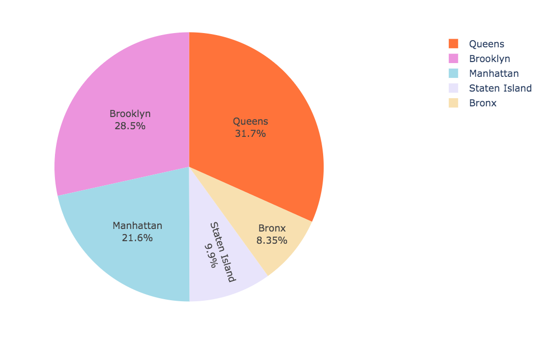
Which New York City’s district do you think has the highest number of property sales?
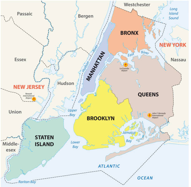
Having visualized the distribution of the real estate sales through the 5 different districts (Queens, Brooklyn, Manhattan, Staten Island, and the Bronx), we noticed a predominance of sales in Brooklyn and Queens with a similar percentage (respectively 28.5% and 31.7%), in contrary to the Bronx and Staten Island which registered only 8.35% and 9.9%.
This is a general point of view, let’s now examine sales trend, for every borough, during the period from 2016-09-11 to 2017-09-03:
It is visible that Brooklyn and Queens are in the higher positions, but additionally, now it is also easy to detect their patterns which are quite similar for the entire period, and to record lower values in 2017-08. Regarding the Bronx and Staten Island, the values are also quite similar. It is worth to notice that after 2017-07 Staten Island, which was always on top of the Bronx, fails.
What about the gross square feet?
We found out that the apartments with higher gross square feet are principally sold in Manhattan, not in Staten Island and Queens where the most vended houses have low gross square feet.
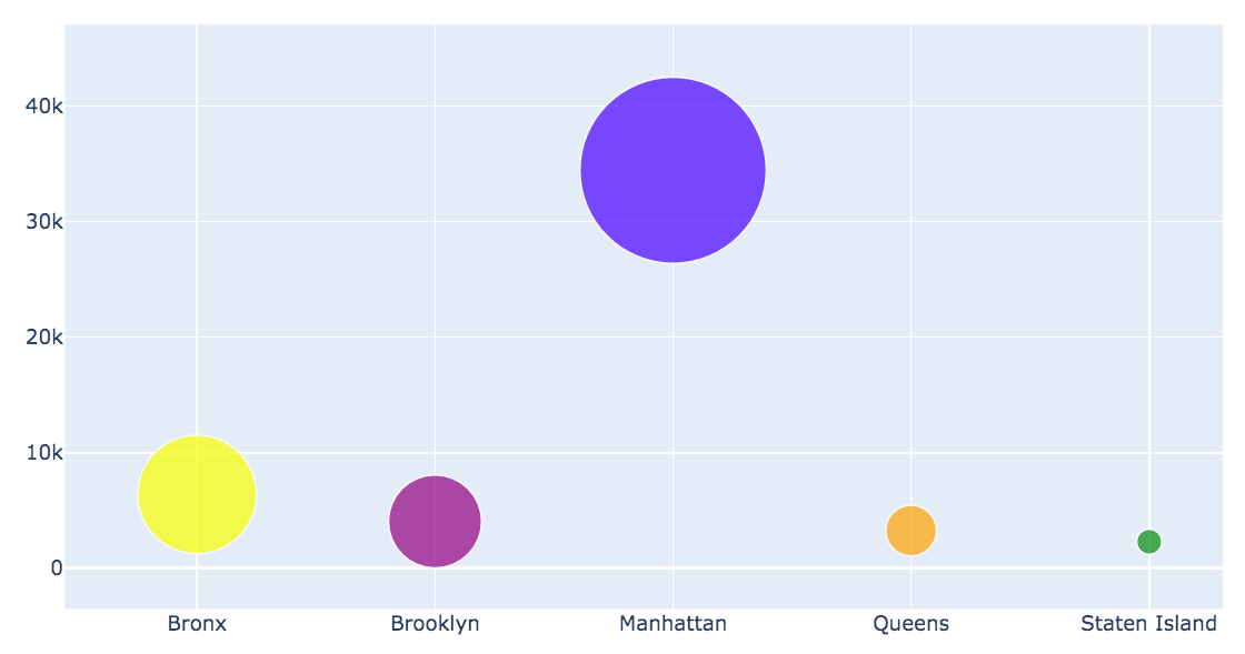
Manhattan seems to win in this case. It is indeed famous for being the most trendy, expensive area. It is characterized by the presence of imposing and luxurious skyscrapers. Can it stem from the assumption that Manhattan is an accessible place to live only for affluent and very rich people (percentage of poverty in Manhattan is only 6.07%), who also can buy a bigger house? Let’s check how prices change between boroughs!
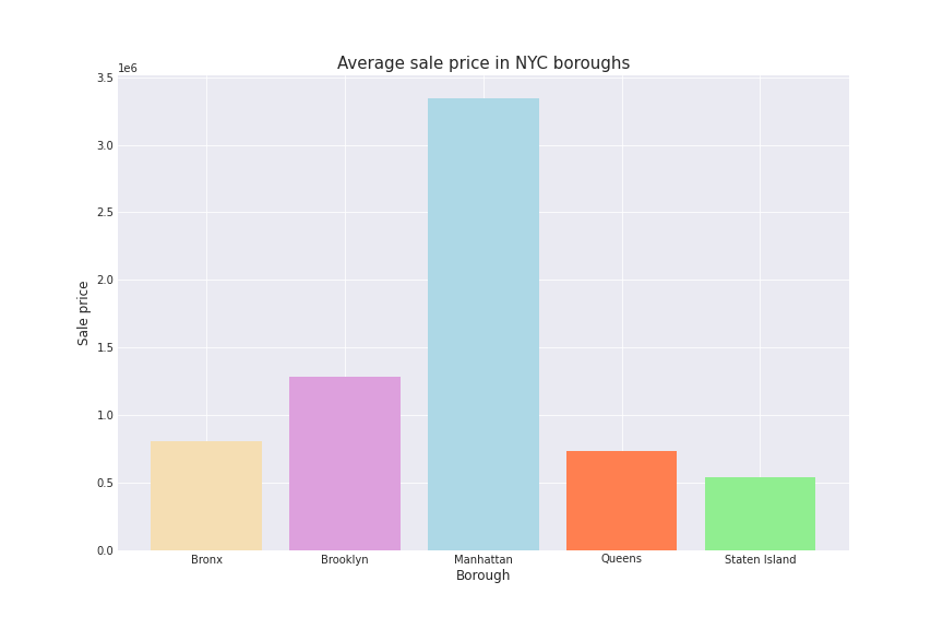
Well, seems to be exactly what we supposed. Bigger houses implicated higher prices and these one seems to be mostly buyed in Manhattan, the costly city!
Now let's move to the real analysis part - designing AR model with Google Trends!
About us
Aleksandra Kukawka
Computer Science / Warsaw University of Technology

Mihaela Diana Zanoaga
Life Science Engineering / EPFL

Bartlomiej Binda
Computer Science / Warsaw University of Technology

Prediction
Seasonal adjustment - preparing dataset for AR model
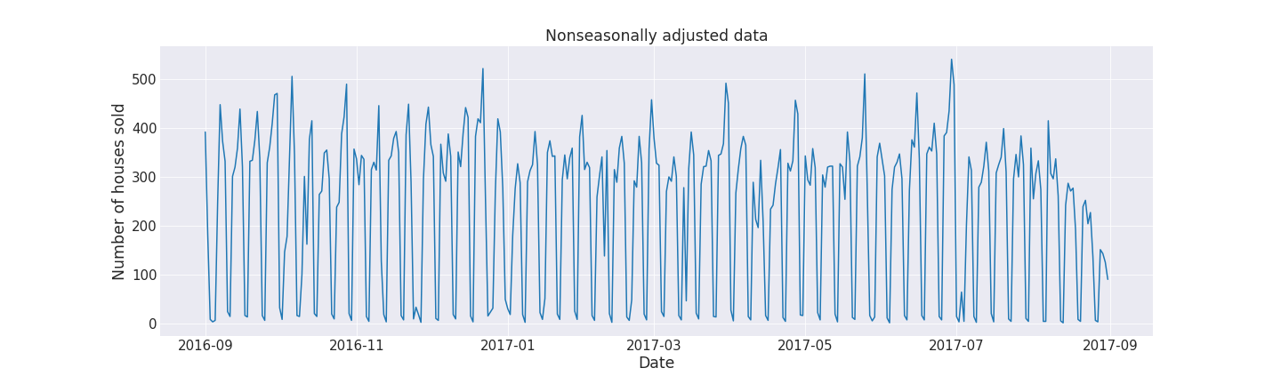
After preprocessing data (removing useless features, removing duplicates etc.) we obtain our required feature - the number of houses sold in New York City for each day in the data frame. At this point, the raw data with the counts bought had to be also adjusted. First of all, during the weekends there were almost no transactions present and hence so many ups and downs on the plot below. This is most likely due to the fact that notaries usually don’t work during the weekend, so the formal signing of new ownership happens during the weekdays.
This is how the non-seasonally adjusted data looks like.
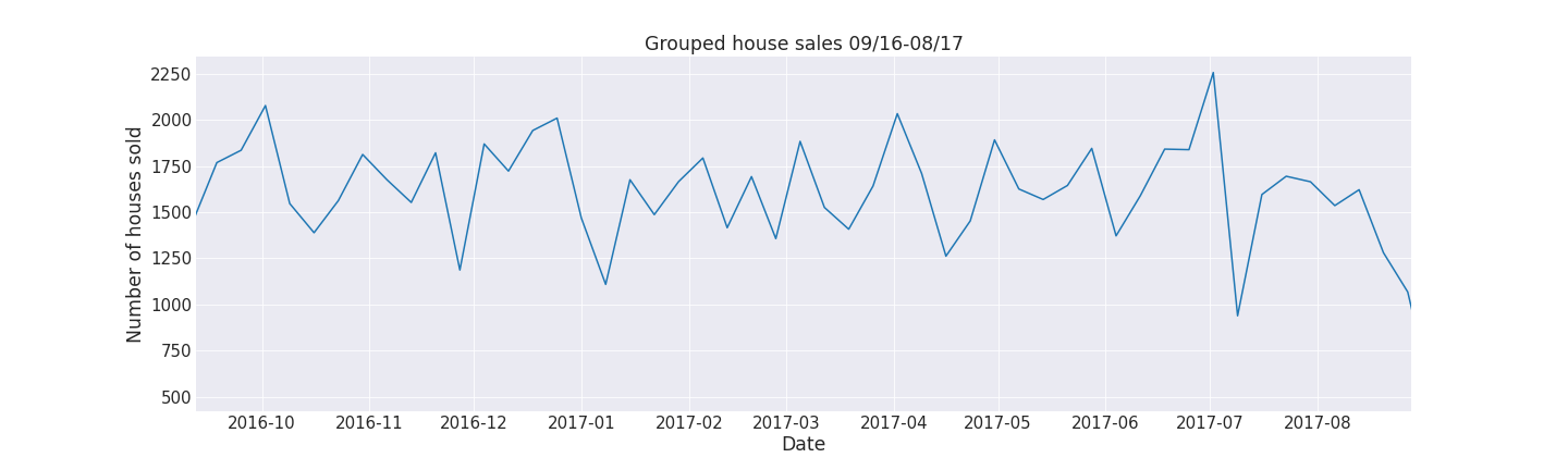
Our initial idea to remove the noise was to simply group the dates in weeks and aggregate the count of total properties sold. However, we weren’t satisfied with the results and as presented below we could still get a better overall trend from the data.
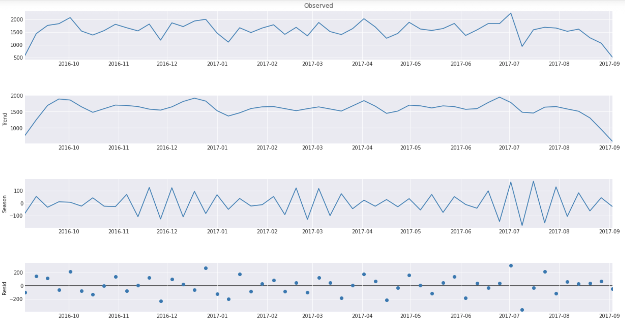
Just like in the Google Trends research paper we opted to use STL for better seasonal adjustments. We wanted the data formatted to weeks starting by Sunday so we use the plot above and extract only the trends to our final data frame that will be used for further analysis (second plot from top).
This is our visualized dataset for an Autoregressive model.
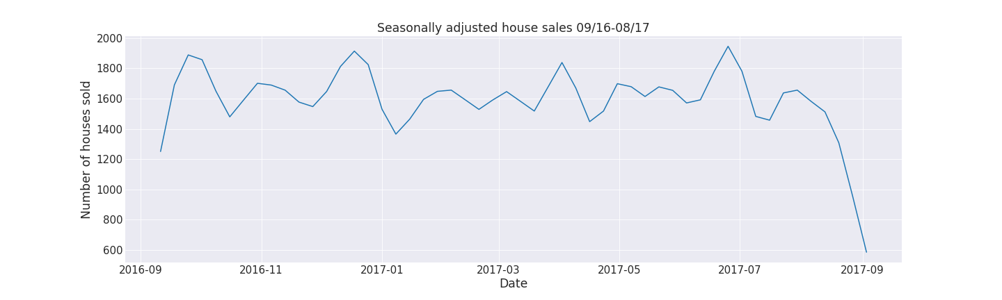
Please note that for almost all the trends we can see that there is a plunging trend at the end of the period. This isn’t due to some turning point but because we aggregate the weeks together and the last week doesn’t contain all 7 days, so the value is thus lower. That’s why further analysis and explaining the AR model last week will not be presented along with the trends.
AR model with and without Google Trends
To predict the real estate sales, we compute an autoregressive model.
The first question we posed ourselves was which lags should we use. To solve that we used the function ar_select_order from statsmodels library which allows us to find the optimal lag structure.
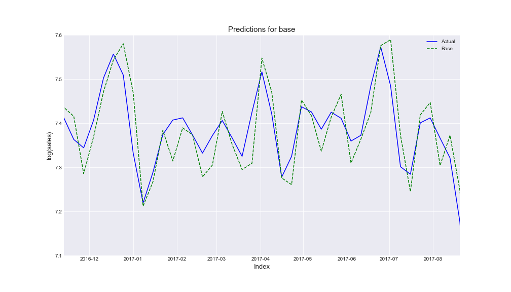
Firstly, we realized the Autoregressive model only with base bata and we considered as lags the first five ones. That is the prediction we obtained:
Following we created again the Autoregressive model, but now adding different sets of Google Trends queries.
To explore the data from Google Trends, we used Google Trends Anchor Bank created by EPFL Data Science Lab. This made our work with Trends data much easier since we didn’t have to download a .csv file for every query and it saved our time.
As we mentioned, we aimed to demonstrate whether Google Trends could represent a reliable mean for improving the predictions, so we tried to find such queries that the prediction including Trends data is better than without. How did we check that? To keep it simple - for every set of queries, we checked the overall improvement (that sometimes wasn’t even here). This is our story of finding the best queries.
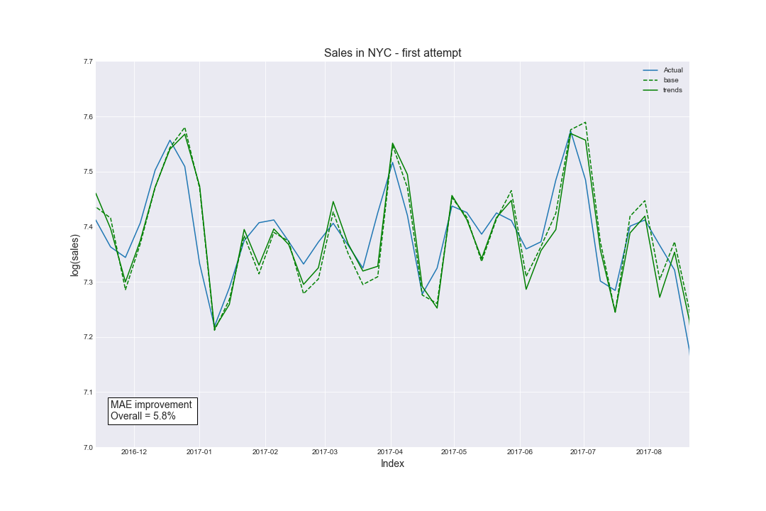
The first attempt:
Our first set of queries arose from brainstorming within the team. We just found a couple of keywords that we found the best: property and real estate. We chose matching lags and tried to compute the prediction’s improvement. And yet - there was, but only 5.8%. We thought that maybe we should use more queries to see the satisfactory value? So, here comes…
The second attempt:
This time we decided to use the same queries as before, but we added to them the two fresh ones. Our set of queries looked like this: property, real estate, mortgage, and houses for sale. We changed the queries in our prediction and now the improvement occurred! We were really happy and we thought that we got this because it was 10.5%. However, we decided to try again to see if we are able to obtain better results.
The third attempt:
This time we changed our strategy - if we wanted to buy a property in New York, where would we search? The answer is obvious - on the websites dedicated to selling properties. Thus, we searched for such websites and chose one of the most common ones: MLS.com. Then our set of queries was: property, real estate, mortgage, houses for sale, and MLS. But the improvement decreased by ~0.1%. So we tried again.
The fourth attempt:
Again - we changed our strategy. But this time we decided to find the information that people search for in Google when they want to buy a house? We typed into Google this exact phrase and we found this interesting webpage with popular real estate keywords. By an experiment, we found the best set so far which consisted of property, realtor, houses for sale, homes for sale, and MLS. The improvement was the largest that we have ever obtained - 14.1%!
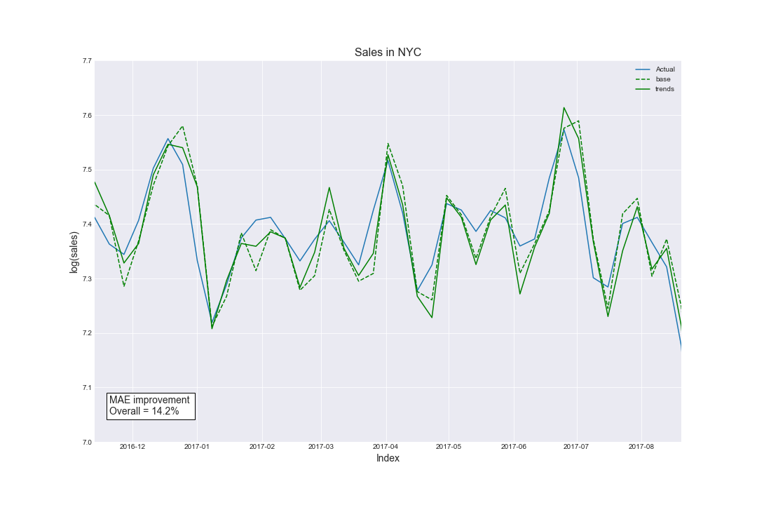
The final attempt:
After some little experimentations, we noticed that the ‘mortgage’ benefits our prediction. Thus, we decided to add it at the end. Therefore, our current set of queries is: property, realtor, houses for sale, mortgage, homes for sale, and MLS. After choosing the best possible lags, the overall improvement of the prediction is 14.2%.
To compute the overall improvement, we computed mean absolute errors for both prediction for base and prediction for Trends. With these values, we could easily obtain the improvement by calculating the difference between them and dividing the difference by mean absolute error for the base.
To conclude, this is the comparison of our first and final attempts. Take a look at what we achieved by choosing appropriate queries and lags in the Autoregressive Model!
Here's the final part of the analysis.
Summary
3 key takeaways
- Choosing appropriate Google Trends queries matters a lot!
We clearly described in the Prediction section how crucial is to choose the appropriate Google Trends. We could not stop after our first attempt because there was even no improvement in the prediction. As you saw, we keep trying and trying. Finally, after several different attempts, we boosted our improvement from ~5% to ~14%! That is why choosing appropriate Google Trends (and obviously - lags) matters a lot. At first, we thought that our starting set of queries would be the best - how wrong we were! It demanded from us a lot of additional research. We had to ask ourselves questions like: what would we search? Maybe others would search in the other way? What are the keywords in marketing strategies regarding selling properties? In the beginning, we didn’t even think about such questions and they occurred to be the most important part of this stage.
Only after the whole process of choice, we could state that a seasonal AR model that includes Google Trends queries is better than this without. Since Google Trends data is available for everyone, it can be used by everyone for forecasting near-term values of economic indicators. And be very helpful.
- When preprocessing data we need to remove seasonalities and look for major trends
Preprocessing is one of the crucial stages of data analysis. Forgetting about steps like removing duplicates for data or null values can impact our end results and show some inconsistencies. Furthermore, when using Google Trends to strengthen our model we should look for turning points and major trends, because these will usually be also better reflected in the Google Trends data. To find the trends it’s best to remove seasonality and to achieve this we recommend STL from statsmodels or R language.
- New York, New York...
From the unprocessed data about sales in NYC and raw queries extracted from Google Trends, we obtained a really useful model that could help real estate agencies to predict short-term property sales in New York City and prepare marketing strategy before the “boom” on the property market. We explored a really big set of data with different crucial (and less crucial) features. As we saw, even the number of sold properties is terrific! It was not easy to preprocess this whole dataset. That only confirms the single thought with which we would want to conclude our whole work:
“New York is not a city. It’s a world.”
Thank You for following this data story. We hope you've learned something on the way!
For more information about authors click here.